The purpose of this lab is to take our robot apart and install the motor driver so we can control the motors directly using our Artemis board, instead of the inaccurate remote. We also explore the option to control the virtual robot that we set up in lab 3 via Python in Jupyter Notebook.
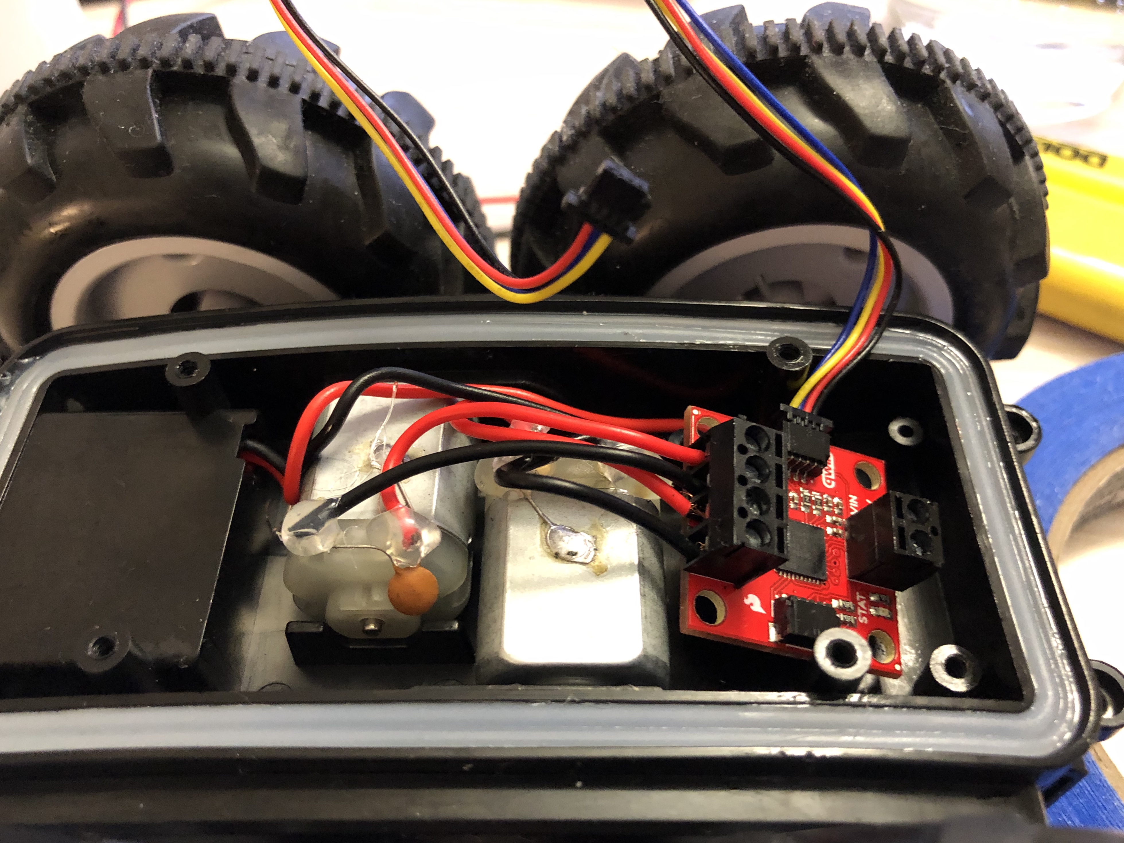
After removing the control PCB and cutting off all the wires, I had to strip the wires using a wire cutter since I don’t have a wire stripper. This turned out to be pretty difficult, especially since the wires are stranded and easy to cut through. Following the hookup guide for the motor driver, I then connected all wires to the motor driver, including \( V_{in} \) and \( G \mkern-2mu N \mkern-2mu D \) from the battery and the four terminals for the two motors. The inside of the car looks like this after all wiring.

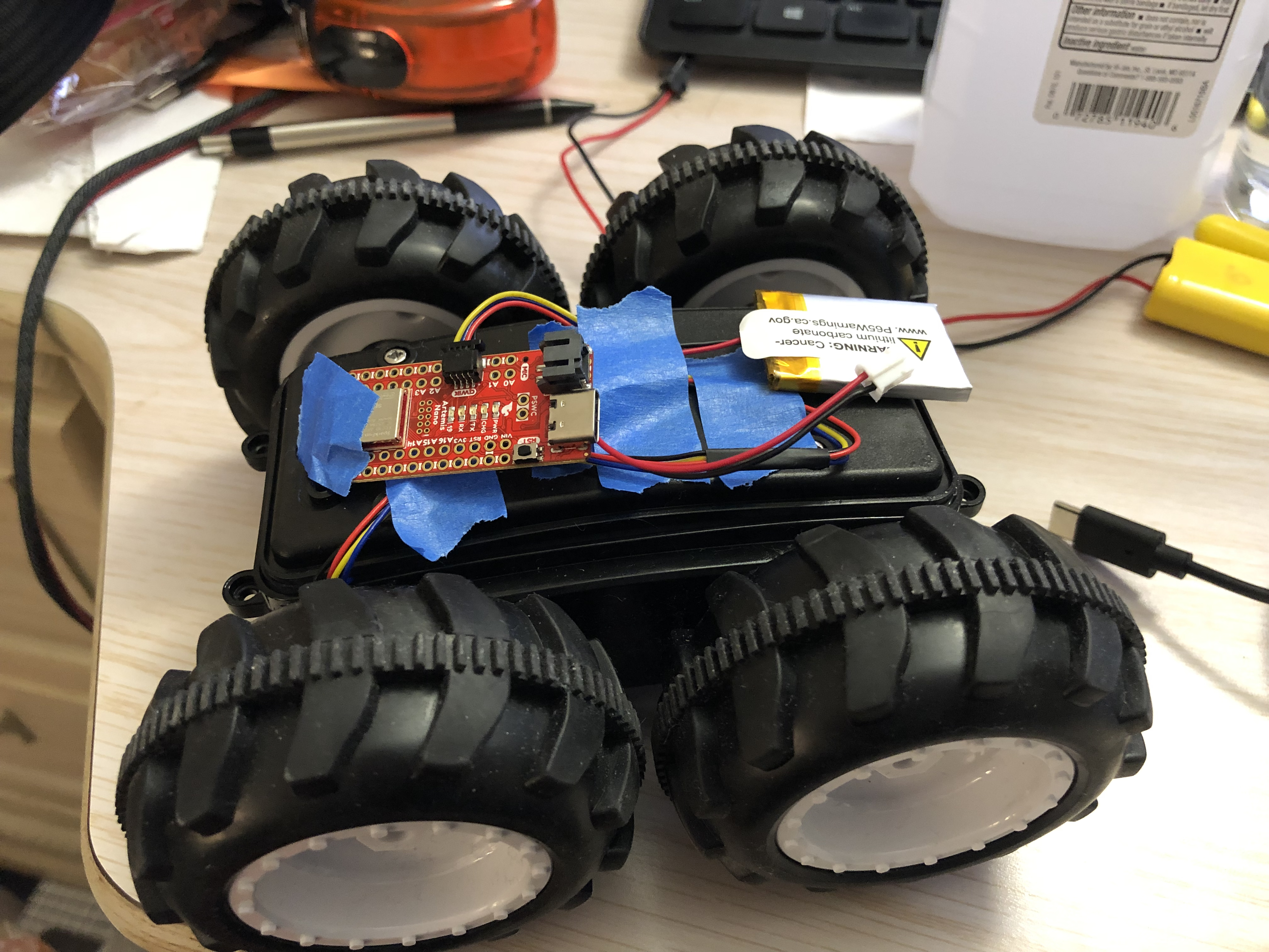
With everything connected, I reassembled the car with the motor driver inside. Unfortunately, I was not able to route the Qwiic connector through the hole as suggested. Instead, I loosely tightened the screws and allowed the connector to come out from the side. The outside of the car looks like this after putting everything in place.

Since there are no holes for me to mount anything, everything is held together by tape. Hopefully, there is a better solution that I can switch to in the future.
With everything connected, I first started running the wire example, which tries to transmit to every I2C address and determine if a device exists according to the response.
nDevices = 0;
for (address = 1; address < 127; address++)
{
	// The i2c_scanner uses the return value of
	// the Write.endTransmisstion to see if
	// a device did acknowledge to the address.
	Wire.beginTransmission(address);
	error = Wire.endTransmission();

	if (error == 0)
	{
	  Serial.print("I2C device found at address 0x");
	  if (address < 16)
	    Serial.print("0");
	  Serial.print(address, HEX);
	  Serial.println("  !");

	  nDevices++;
	}
	else if (error == 4)
	{
	  Serial.print("Unknown error at address 0x");
	  if (address < 16)
	    Serial.print("0");
	  Serial.println(address, HEX);
	}
}
if (nDevices == 0) Serial.println("No I2C devices found\n");
else Serial.println("done\n");
By running this, I found out that the motor driver occupies the address 0x5D, which matches the default configuration given by its documentation.

The next step is to control the motor. This is achieved by setting the direction and the magnitude for a certain motor after configuring its command interface, I2C address, chip select pin, inversion mode (depending on the arbitrary selection of orientation as well as how the motor terminals are wired), etc. The following code, for example, drives the robot forward at full speed.
//pass setDrive() a motor number, direction as 0(call 0 forward) or 1, and level from 0 to 255
myMotorDriver.setDrive( LEFT_MOTOR, 0, 255);
myMotorDriver.setDrive( RIGHT_MOTOR, 0, 255);
I tested different values to find out what the minimum value that can move the wheels without load is. First, I set both motors to a level of 65 and alternate the direction. The turns are very inconsistent as we can see.
70 was then tested. It performed a little better, only missing a few turns, but it’s still not what we want.
Finally, when the value is set at 75, both wheels turn consistenly without glitches.
However, this experiment is under ideal conditions without any load. When I put the car on the floor, I found out that I need to set the level to 100+ depending on the surface for it to run consistenly.
Another problem with these cheap motors is that they have different accleration and top speed. In my case, the left motor accelerates better (relatively, as in the left motor has a higher acceleration when both motors have the same top speed) but the right motor has a higher top speed. Therefore, I conducted a few experiments hoping that I would find an ideal scaling factor that balances the two motors, but the best I can do is still underwhelming. The car sort of follows a straight line for the first 2 meters because I indirectly adjusted the acceleration for the right motor by setting the maximum speed to 90% of what the left motor has. However, the top speed takes over after the acceleration phase, which is why we see the car slighly go towards the right at first but eventually turned to the left. In the future, we have to account for that when controlling the robot.
Just for fun, I integrated the motor control code with the FFT code from lab 1. Four different frequencies are used for four different motions: 300Hz -> straight forward, 400Hz -> spin counterclockwise, 500Hz -> spin clockwise and 600Hz -> straight backward. Each frequency has an error margin of ±20Hz, partly because the resolution of FFT is set at about 11Hz. I used a tone generator on my phone to control the car to move around in my kitchen.
As we can see, the motion is quite jittery. However, this is not a control issue but rather a noise issue. Whenever the motors run, they change the loudest frequency to approximately 1.1kHz as they are right next to the Artemis board and the weak speaker on my phone cannot compete with that, which is why sound is not an ideal means to control our car. It is pretty fun to play with though.
For this part of the lab, we run the setup script from the lab 4 base code and start lab4-manager as well as a Jupyter Notebook server that allows us to control our virtual robot by setting its linear and agular velocity using Python. Since we have access to Python, we have much better control of the robot in terms of timing and setting the exact velocities, which means having the robot traverse a square is incredibly simple.
The code that controls the motion of the robot is shown on the right. From lab 3, we know that the maximum angular velocity that the robot can handle is \( \frac{\pi}{2}\,rad/s \), which is why setting the angular velocity to 2 effectively makes it rotate \( 90^{\circ} \) every second. The linear velocity is also set at 2, which forces the robot to travel at its maximum linear velocity, \( 1m/s \). It therefore unrealistically follows a perfect square.