Using the provided Bayes filter implementation, we try to perform actual localization using the real robot.
First, I wanted to try the provided implementation and see if it performs differently compared to my own implementation. The provided implementation is shown on the left and my own on the right for reference.
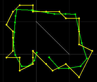
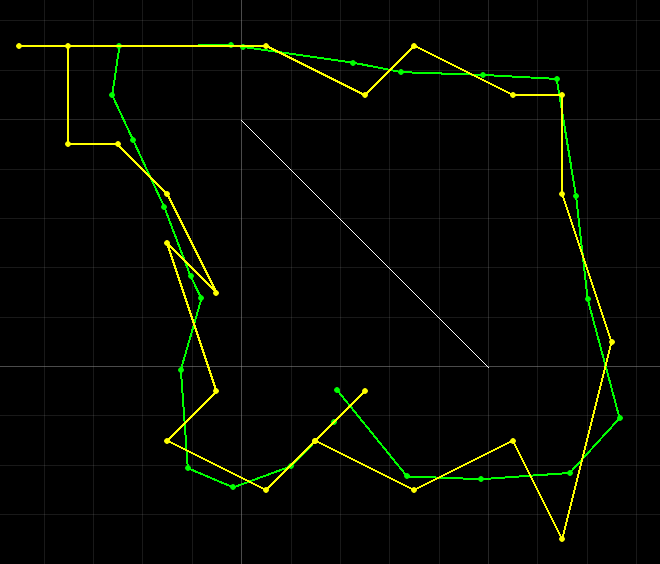
As we can see, both do a passable job when it comes to localization for this particular map gemotry. Before I start gathering observation data from the real world, however, I wanted to check how the filter performs on the actual layout of my room.
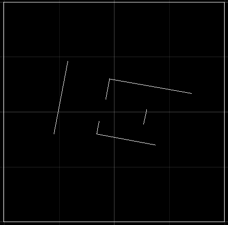
First, I replaced the prediction step with init_uniform_distribution() so that the prior belief (bel_bar) is a uniform distribution. Therefore, for every step, only update step is calculated.
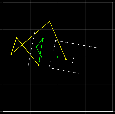
The result is quite disappointing. The only two points that got close are the origin and the one on the top. I then tried to incorporate the prediction step back.
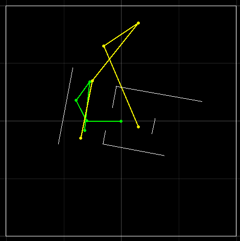
Similarly, the only points that the Bayes filter got right were the first and the last two points. The map geometry is ultimately to blame here. It is too simple due to how tiny my apartment is and the bounding box for the simulator definitely did not help as the boundary is easily mistaken for the actual walls in real life. However, if I enlarge the bounding box to create an asymmetry, maybe the result will improve. This turns out to be a fool’s errand.
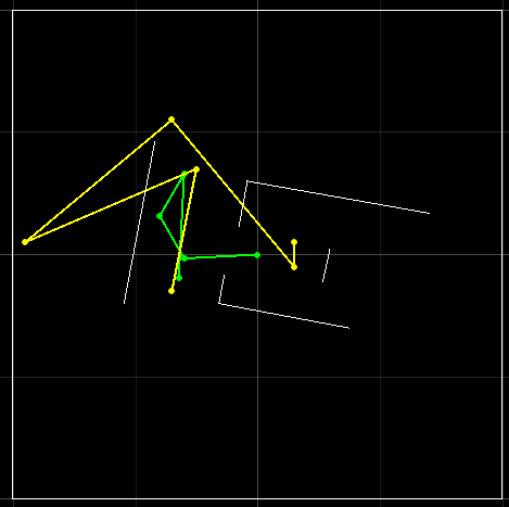
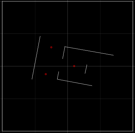
In the image above, the bounding box is set to 3x3 (not shown on the plotter). The result running both prediction and update is very similar to the ones before. I also tested different sizes and none helps. The points that are more accurate than others are near the origin and in the hallway away from the entrance (marked in the map below). The problem is that the hallway is entirely covered by carpet, which means that the robot cannot really spin to gather distances at different angles. Therefore, I am not optimistic about real-world localization.
For the real robot, the procedure is very similar. By creating an additional command called scan, the robot can send 72 bytes of data (array of 18 4-byte ints) back to the VM after performing a scan. With the distance data, the provided init_bayes_filter can be used to find the most probably location of the robot. I tested it by placing the robot at several measured locations, and below are the results. On the left are the ground truth location and the Bayes filter location. On the right are the data points plotted on polar coordinates.
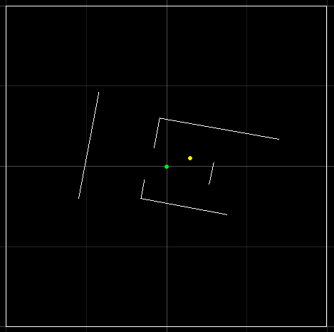
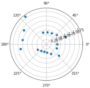
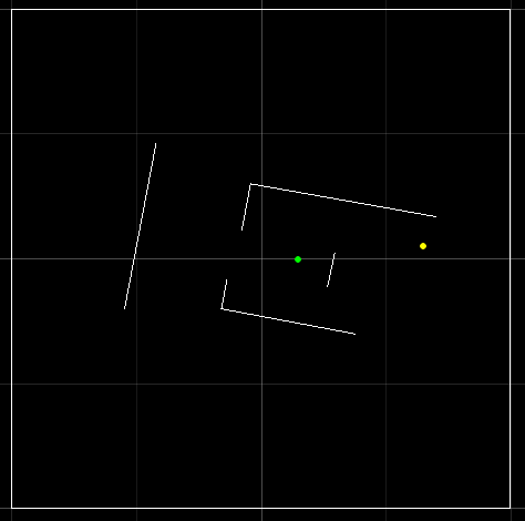
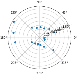
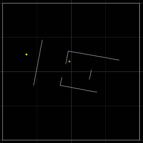
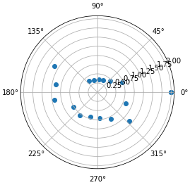
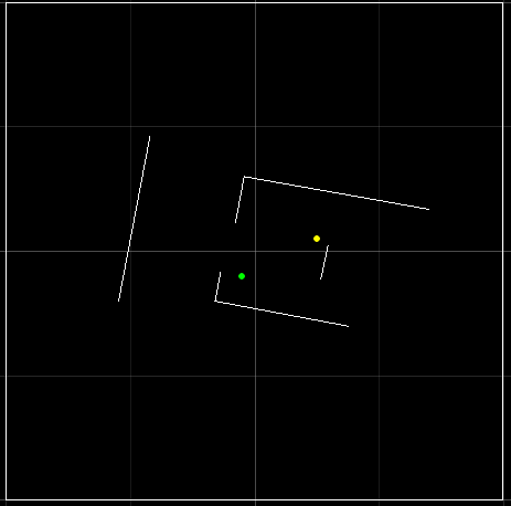
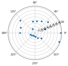
This pretty much matches the expection from earlier. When the robot is at the origin, the prediction is relatively accurate. However, when we move it away, the predictions go all over the place. A major cause of this is the simple geometry of the map but I have very limited floor space to work with. Another source of error is the inaccuracies in the angle measurments. Since there are several cliffs on this map, a tiny error in degrees near these cliffs can create a huge difference when calculating the probability. I also made a mistake in my implementation that I only realized afterwards. Since I used radian instead of degree in my yaw calculation, I calculated the step between scans incorrectly. Instead of scanning every 20 degrees, it was closer to 21.18 degrees. I fixed it for the last location but it didn’t really help much since the angle was off regardless. With a more complex and continuous geometry, I believe the agorithm could perform much better.