Following the instructions from the given Jupyter notebook, I implemented the following five functions that represent five different components of each step of the Bayes filter.
First, we calculate the relative motion parameters, which are two rotation angles and a translation distance, from odometry readings.
# In world coordinates
import math
def compute_control(cur_pose, prev_pose):
    """ Given the current and previous odometry poses, this function extracts
    the control information based on the odometry motion model.

    Args:
        cur_pose  ([Pose]): Current Pose
        prev_pose ([Pose]): Previous Pose

    Returns:
        [delta_rot_1]: Rotation 1  (degrees)
        [delta_trans]: Translation (meters)
        [delta_rot_2]: Rotation 2  (degrees)
    """
    cur_x, cur_y, cur_a = cur_pose
    prev_x, prev_y, prev_a = prev_pose
    delta_trans = ( (cur_y-prev_y)**2 + (cur_x-prev_x)**2 )**0.5
    deg = math.atan2(cur_y-prev_y, cur_x-prev_x)
    delta_rot_1 = deg - prev_a
    delta_rot_2 = cur_a - deg
    return delta_rot_1, delta_trans, delta_rot_2
Then, we calculate the probability that the robot reaches an arbitrary pose given the previous pose and the control parameters.
# In world coordinates
def odom_motion_model(cur_pose, prev_pose, u):
    """ Odometry Motion Model

    Args:
        cur_pose  ([Pose]): Current Pose
        prev_pose ([Pose]): Previous Pose
        (rot1, trans, rot2) (float, float, float): A tuple with control data in the format
                                                   format (rot1, trans, rot2) with units (degrees, meters, degrees)

    Returns:
        prob [float]: Probability p(x'|x, u)
    """

    del_rot1, del_trans, del_rot2 = computer_control(cur_pose, prev_pose)

    p1 = loc.gaussian(del_rot1-u[0],0,loc.odom_rot_sigma)
    p2 = loc.gaussian(del_trans-u[1],0,loc.odom_trans_sigma)
    p3 = loc.gaussian(del_rot2-u[2],0,loc.odom_rot_sigma)

    prob = p1 * p2 * p3
    return prob
With that probability, we multiply that with the probability that the robot was indeed at that pose in the previous time step, and sum all these possibilities together for each possible pose to obtain a probability map of the robot’s current pose.
def prediction_step(cur_odom, prev_odom):
    """ Prediction step of the Bayes Filter.
    Update the probabilities in loc.bel_bar based on loc.bel from the previous time step and the odometry motion model.

    Args:
        cur_odom  ([Pose]): Current Pose
        prev_odom ([Pose]): Previous Pose
    """
    u = compute_control(cur_odom, prev_odom)
    for i in range(Mapper.MAX_CELLS_X):
        for j in range(Mapper.MAX_CELLS_Y):
            for k in range(Mapper.MAX_CELLS_A):
                loc.bel_bar[i,j,k] = 0
                for i1 in range(Mapper.MAX_CELLS_X):
                    for j1 in range(Mapper.MAX_CELLS_Y):
                        for k1 in range(Mapper.MAX_CELLS_A):
                            loc.bel_bar[i,j,k] += loc.bel[i1,j1,k1] * odom_motion_model((i,j,k),(i1,j1,k1),u)
We can also calculate the robot’s possibility at an arbitrary pose by scanning its surroundings. We use the scanned data and the ground truth data at a certain pose to calculate the probability array indicating the likelihood that the robot is indeed at that pose.
def sensor_model(obs, cur_pose):
    """ This is the equivalent of p(z|x).


    Args:
        obs ([ndarray]): A 1D array consisting of the measurements made in rotation loop

    Returns:
        [ndarray]: Returns a 1D array of size 18 (=loc.OBS_PER_CELL) with the likelihood of each individual measurements
    """
    prob_array = np.zeros(loc.OBS_PER_CELL)
    views = Mapper.obs_views[cur_pose[0],cur_pose[1],cur_pose[2]]
    for i in range(loc.OBS_PER_CELL):
        prob_array[i] = loc.gaussian(views[i]-obs[i],0,loc.sensor_sigma)
    return prob_array
Finally, we multiply the probability calculated from the prediction step with the probability given by the sensor model, which gives us a more accurate probability map.
def update_step():
    """ Update step of the Bayes Filter.
    Update the probabilities in loc.bel based on loc.bel_bar and the sensor model.
    """
    loc.get_observation_data()
    obs_data = loc.obs_range_data()
    for i in range(Mapper.MAX_CELLS_X):
        for j in range(Mapper.MAX_CELLS_Y):
            for k in range(Mapper.MAX_CELLS_A):
                acc = 1
                prob_array = sensor_model(obs_data, (i,j,k))
                for l in range(loc.OBS_PER_CELL):
                    acc *= prob_array[l]
                loc.bel[i,j,k] = loc.bel_bar[i,j,k] * acc
    loc.bel /= np.sum(loc.bel)
By spinning the robot and recording the distance readings from the time-of-flight sensor, I got the mapping below plotted in polar coordinates. To check the reliability of the yaw calculation as well as the data from the TOF sensor, this plot consists of data from three consecutive rotations.
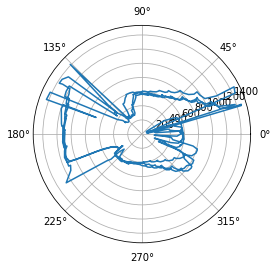
This is actually not too bad. For reference, here’s the actual room that I measured, with an added box.
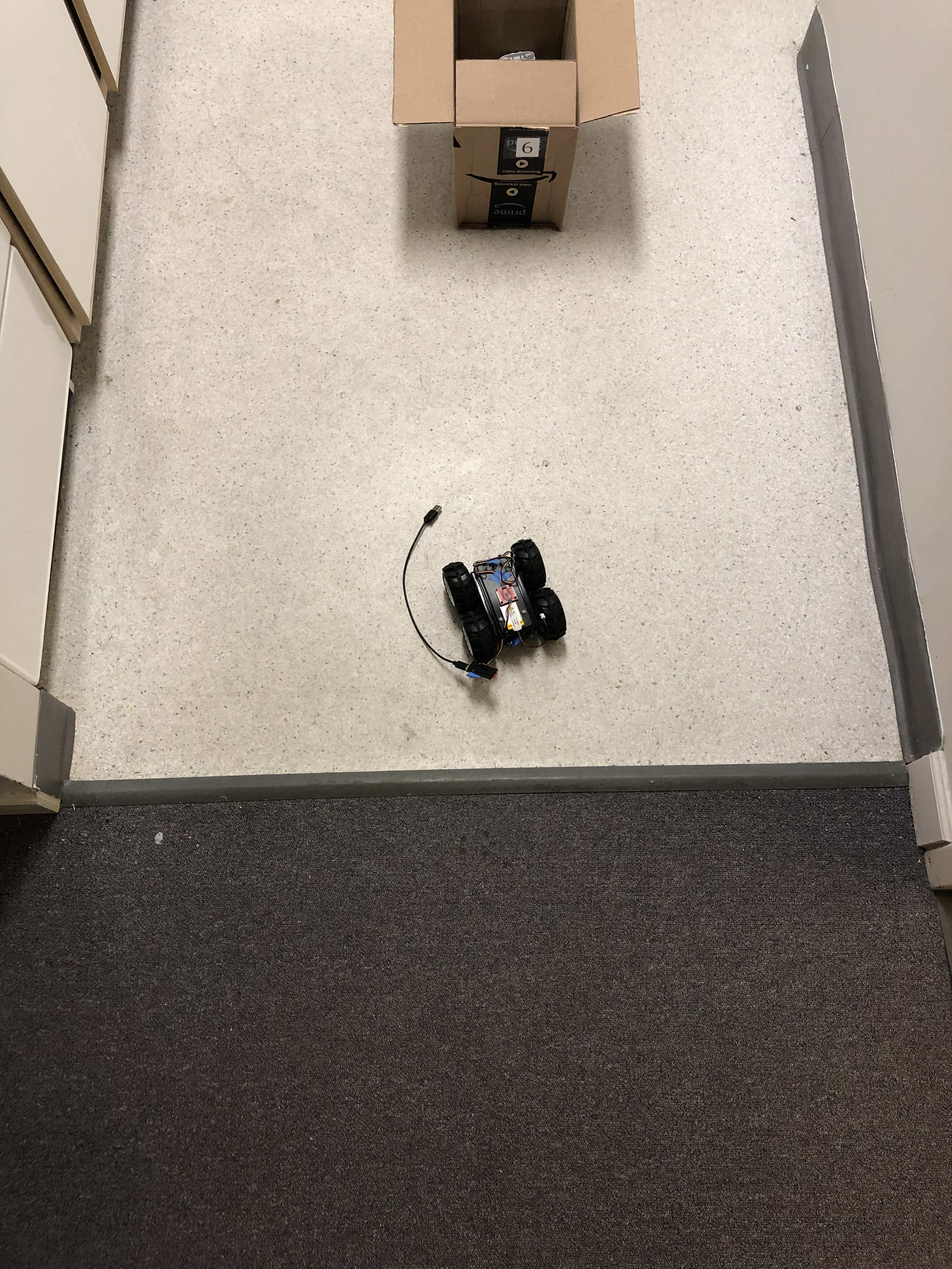
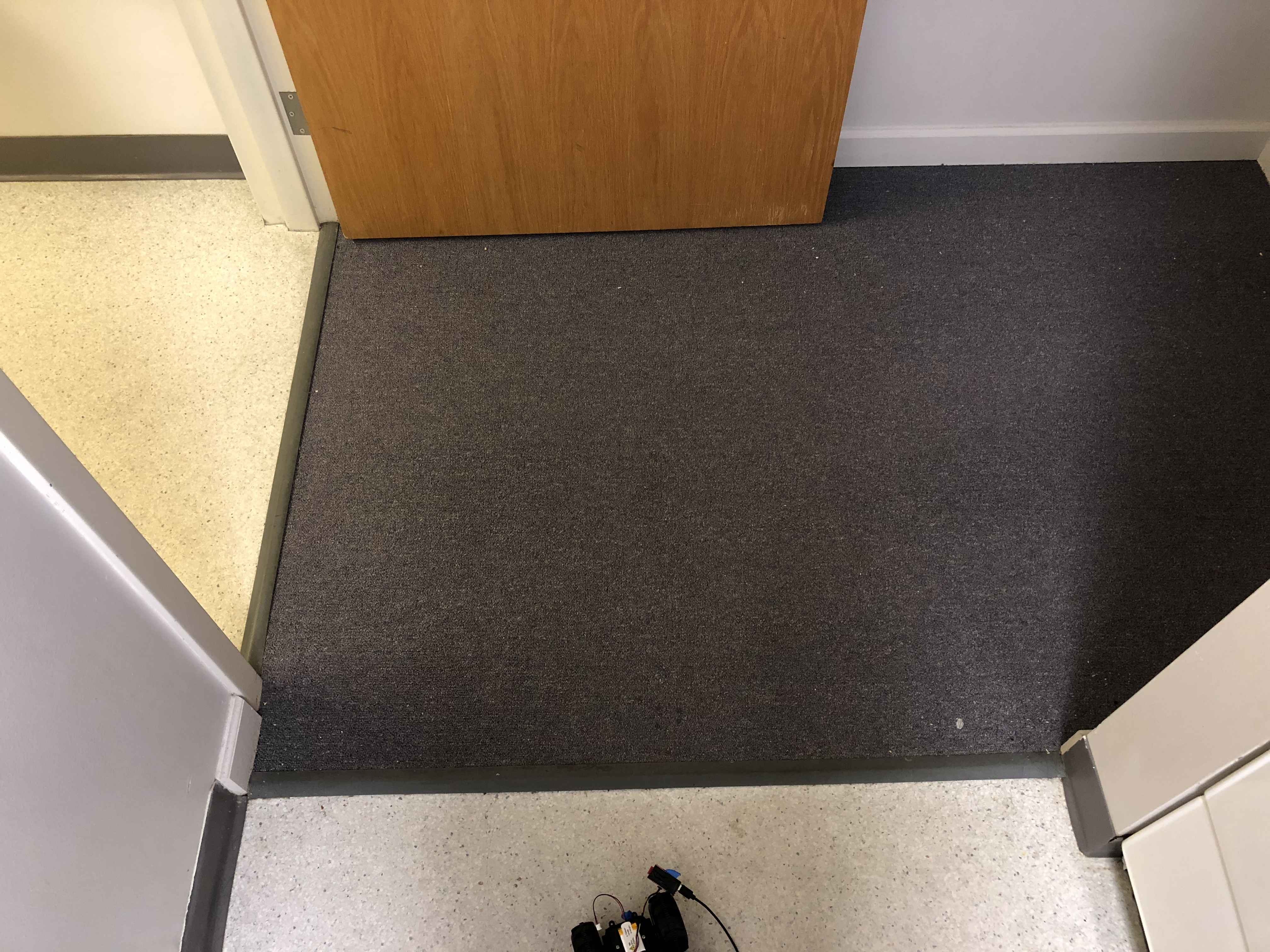
We can see that the box is detected on the right hand side of the plot, even though it is very noisy. The corners are detected surprisingly well, and the left hand side of the plot matches what the robot could see at that position.
One thing that I did notice is that the robot became a little more jittery, probably because it was waiting for the sensor data. This can be easily fixed by simply skipping that iteration if the TOF data is not ready.
Using the same data, we could calculate the transformation matrices and convert the distance as well as the yaw to an actual point in the room’s coordinate system.

Since \( \psi \) in \( T_R^i \) is the only non-zero angle in the entire equation, it becomes the equation below if we ignore the z component.

To perform a sanity check, I calculated a few values by hand when the robot is at different angles, and the values check out. Then, using this matrix, I plotted the data from one rotation in Cartesian coordinates.
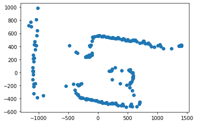
As expected, they have the same shape. This is then plotted to the plotter.
