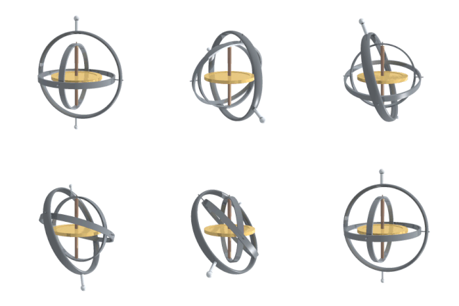
The next step in feedback control is to determine where our robot is, and what direction is facing. We can achieve this by setting up the IMU which contains an accelerometer, a gyroscope, and a magnetometer. Using data from these sensors, we can determine the approximate odometry of the robot.
As per the instructions, I installed the library for the IMU and scanned the I2C address of the IMU, and it’s 0x69 as expected. When running the example script, I tried to apply acceleration on all three axes of the accelerometer as well as all three axes of the gyroscope.
As we can see, I was oscillating the IMU first on the accelerometer’s X, Y, Z axes and then on the gyroscope’s Z, X, Y axes, in that order with each axis specified by a color on top. The accelerometer outputs don’t have a maximum range that my arm could produce but the outputs from the gyroscope are capped at around 250.
Using the the following equations, we can calculate the pitch and roll of the IMU when the only acceleration applied on the accelerometer is gravity.
\[ pitch=atan2(\frac{a_x}{a_z})\] \[ roll=atan2(\frac{a_y}{a_z})\]
I then tested the code by pressing the accelerometer onto a vertical surface, turning it 90 degrees each time, and plotting the outputs.
The roll and pitch both start at 0 degrees. Then, the pitch goes to \( -\frac{\pi}{2}rad \), the roll goes to \( -\frac{\pi}{2}rad \), the pitch goes to \( \frac{\pi}{2}rad \), and the roll goes to \( \frac{\pi}{2}rad \). We can also see that when one output is stable, the other is extremely noisy and inaccurate. This is due to the fact that \( a_z \) approaches 0 when we tilt the IMU 90 degrees. Otherwise, it honestly seems very accurate.
I also recorded the time-domain signals of three different scenarios. 1. An oscillation. 2. Sitting perfectly still at two different sampling frequencies. 3. Short taps/pulses. I then use Python to plot the frequency-fomain signals, wondering if there is a high-frequency peak that I need to get rid of. Here are the results.
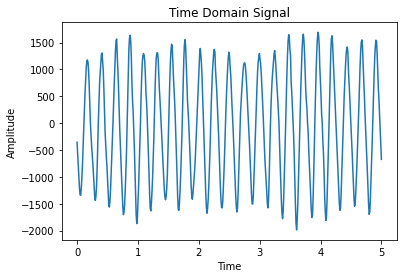
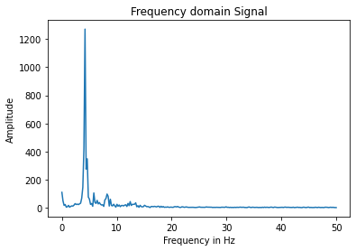
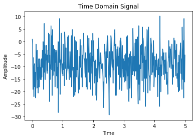
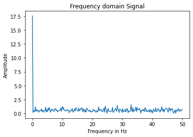
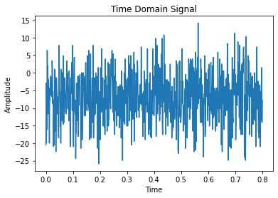
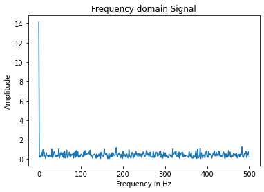
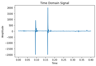
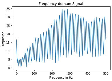
Honestly, nothing is really unexpected in the FFT spectrum. For the first signal, there is a very strong peak at about 5Hz, which matches what we can observe from the time-domain signal. For the second and third signal, the magnitude across all higher frequencies are relatively similar. For the fourth signal, the output also makes sense because the Fourier Transform of the delta function is a non-zero constant. Judging from the results, I don’t believe that there is a specific high-frequency peak that I need to get rid of. Regardless, I implemented a low-pass filter that I will discuss in the filter section.
We can also calculate the roll, pitch and yaw using the gyroscope data. Since we get an angular velocity from the gyroscope, we only have to multiply that by the change in time to get the angular displacement. However, since the process is digital with a sampling frequency, we are bound to lose some accuracy when the movement is sudden or non-linear. The bias in the measurements would also create an error that accumulates over time, also known as the drift.
As we can see from the beginning of the clip, when doing absolutely nothing to the IMU, the position obtained through summation is already drifting. When I rorate the IMU, the gyroscope pitch and roll are very steady while the accelerometer data gets extremely noisy and inconsistent. I tried changing the sampling frequency, and it seems the be doing a little better. However, when we print to serial, that actually becomes a major source of delay, which limits our sampling frequency.
Since the accelerometer data has some high-frequency noise and the gyroscope has a bias, I decided to try to get rid of both. For the accelerometer, I have a weighted sum of the current reading and past readings. For the gyroscope, I simply set a minumum threshold when summing the angular displacement. The results look like this (I seperated pitch and roll so we don’t need to see eight lines at once).
We can see that the noise from the accelerometer is pretty much gone and the drift from the accelerometer is also very minimal. However, it still suffers from the non-linearity as a result of insufficient sampling frequency.
For the yaw, I also have a raw version from the gyroscope and the filtered (cutoff) version. We can come to the same conclusion as above, even though it seems like the yaw does not suffer from the drift as much.
Since both methods have their flaws, I implemented a complementary filter that combines the two sources and see if we can have a drift-less, noise-less output.
The result seems relatively acceptable. It doesn’t have too much noise and the drift is somewhat negligible over a short period of time.
Using the code provided, I calculated another yaw and compared that to the yaw calculated through the gyroscope data.
xm = myICM.magX()*cos(pitch) - myICM.magY()*sin(roll)*sin(pitch) + myICM.magZ()*cos(roll)*sin(pitch);
ym = myICM.magY()*cos(roll) + myICM.magZ()*sin(roll_rad);
yaw = atan2(ym, xm);
The two lines follow the same trend in general, except when the sign of the magnetometer yaw changes from negative to positive. However, the magnetometer data is very noisy and extremely susceptible to magentic inference, which our motors do generate. Therefore, I don’t believe that the magnetometer data is that useful, which is unfortunate, especially since our only data source for the yaw is the gyroscope.
First, I created a ramp function for the motors so that the robot spins in one direction before another and recorded the yaw over the same period of time.
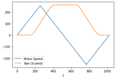
As we can see from the plot, the robot doesn’t start turning at all until the motor value is set to about 120, and the slope only gets stable until the speed hits about 180.
Therefore, when trying to make the robot turn as slow as possible, I set the motor speed to about 180. I also check the yaw so that it would stop after one full rotation.
If I set the motor values to something low, however, only one set of wheels would really work due to the differences in the motors.
Using Arduino’s PID library, I was able to tune my P and I parameters so that my robot turns relatively slowly and steadily with only one set of wheels.
From the video, I measured approximately 6 seconds per rotation.
The motor values and the gyroscope data are plotted below.
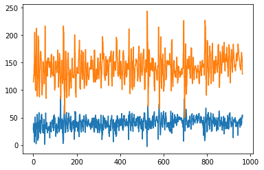
The angular velocity matches my measurement as it is about 60 degress per second.
For this part of the lab, we are trying to see how accurate the odometry actually is. We first set up the lab like all previous labs, then we launch three tools: the simulator, the plotter, and the keyboard teleoperation tool. Then, we plot the location (noisy, untrusted odom as well as the ground truth) of the virtual robot on the plotter continuously while controlling the virtual robot using the teleoperation tool.
while True:
  pose = robot.get_pose()
  gt_pose = robot.get_gt_pose()
  robot.send_to_plot(pose[0], pose[1], ODOM)
  robot.send_to_plot(gt_pose[0], gt_pose[1], GT)
  time.sleep(0.5)
The poses are sampled at 2Hz to prevent overcrowding the plotter. Here’s what the plotted looks like when driving around.
As we can see, the odometry data and the ground truth are somewhat close to each other at the beginning, with the ground truth matching the trajectory exactly (of course). However, as time goes by, they are farther and farther from each other as the noise/error in the odometry accumulates over time. By the end, they are off by at least a few meters.
I also tested the robot in several other conditions. For example, when it is staying completely still.
This video is sped up 80 times. Therefore, in 800 seconds, our robot has effectively traveled around the origin while staying completely still.
Or, when the robot is traveling at max speed.
It doesn’t seem like speed has a significnat impact on the noise.