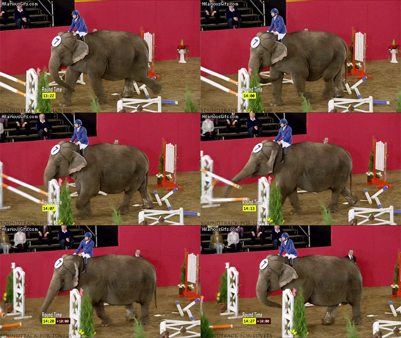
The first and arguably the most essential part of feedback control is obstacle avoidance. After all, we don’t want this to happen to our robot.
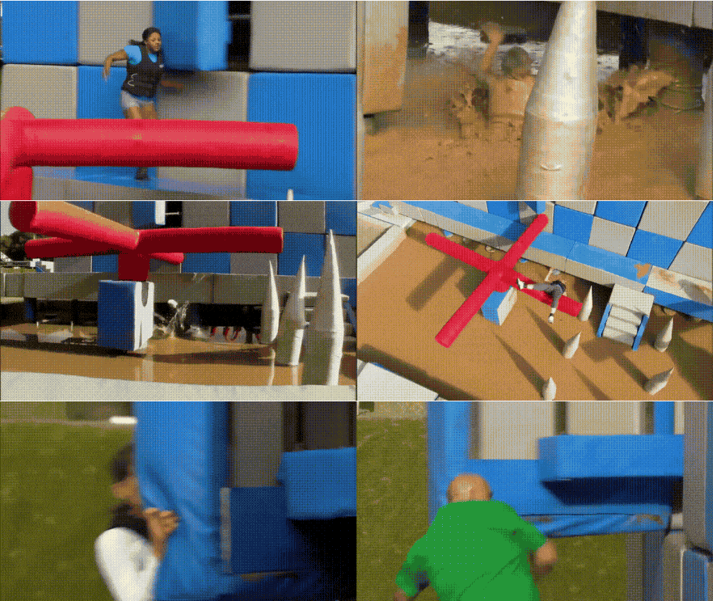
Therefore, by adding two sensors (proximity and distance) to our robot, it will be able to sense anything in front of it and actively avoid the obstacle, either stopping completely or turning away. We also conduct similar experiments in the simulator, but the virtual robot differs from the physical robot in two ways. In the simulator, there is no acceleration, and the robot is very rigid.
Following the instructions from the lab handout, I installed the library, connected, and found the I2C address of the VCNL4040 proximity sensor. It has an address of 0x60, which is its default hard-wired address, as stated in the reference documents.
Using the grid, I was able to conduct experiments mapping the actual distance of objects to the “proximity value,” as seen below, with the left one on linear scale and the right one on log scale.
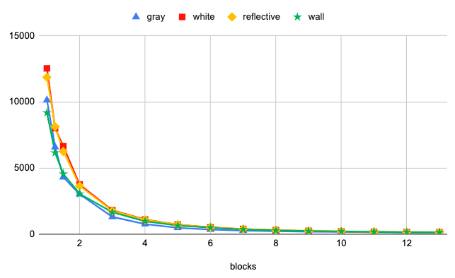
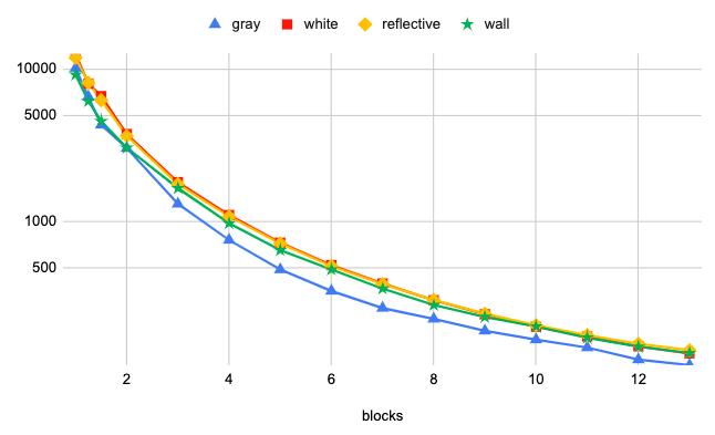
I tested different materials with different colors. Gray and white both refer to front and back of the piece of paper for calibration, while reflective is the rigid piece of paper from the bluetooth adapter that reflects visible lights better. The time between two measurements is about 0.08s, but the proximity value fluctuates a lot before settling down the a final value, which takes about two seconds after the object has moved. Different lighting condition does not really affect the proximity value, bu the ambient light value and the white value are influenced significantly.
As we can see, the proximity value depends on not only the distance but also the material. Its resolution also degrades rapidly for objects merely 5cm away. Therefore, this sensor might not be the best fit for our fast robot as range will be very important.
Similarly, I tested the I2C address (0x29, as expected) and calibrated the VL53L1X sensor using the piece of 17% gray paper by placing it 140mm away from the sensor. I then tested the acccuracy of the time-of-flight sensor by measuring different distances defined by a tape measure. Ref is the reference sensor data with 100% accuracy.
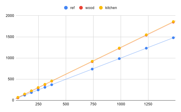
The results are obtained with two surfaces, my bathroom door which is wood, and my kitchen wall. Obviously, the sensor produces higher values for both surfaces, but the results from different surfaces appear quite consistent. Therefore, we can simply apply a scaling factor to convert the sensor data to actual distance.
I also tested the timing of different parts of the code. Namely, functions startRanging(), getDistance(), clearInterrupt(), stopRanging, and the time it takes for the sensor to return a valid distance after startRanging(). startRanging(), clearInterrupt(), and stopRanging only takes \( 455\mu s \), while getDistance() takes \( 725\mu s \). Presumably, this is because the first three functions only send a command while the latter has to request the data as well as reading it. The time it takes for the sensor to return a distance depends on the intermeasurement period, which would depend on the mode we choose. For long ranging mode, it takes about \( 94055\mu s \). For short ranging mode, it takes about \( 28516\mu s \). The two different modes result in different sampling frequencies, 10.6Hz and 35Hz, respectively. For avoiding obstacles, I believe that long ranging mode might be better. The robot only moves 20cm more when waiting for the long ranging data, but we get a much better range, which also means the robot can plan ahead.
For the “roomba”, I don’t believe that the proximity sensor will be of much use. The proximity sensor has a better resolution when the object is only a few centimeters away, but a few centimeters from where the sensors are mounted might not even reach the outer border of the robot. Besides, since our robot is going to be fast, a crash is bound to happen if we pick up something a few centimeters away. The proximity value doesn’t even update until 2 seconds after the change in distance. Therefore, only the distance sensor will be required.
I plan to explore the quickest way to stop the robot completely. One way to stop it will be simply setting the velocity to 0. This is slow but safe. Another way is to put the motors in full reverse, which will definitely result in a flip. Therefore, I need to find a (presumably small) negative velocity that I could apply to the motors so that the motors could decelerate the robot as soon as possible without resulting in a flip, and then bring the velocity up to 0. Since the next lab is about PID control, we can try to use PID then.
Everything else is simple. All we have to do is have the robot driving in full velocity, and when our time-of-flight distance sensor detects a distance that is slightly above our braking distance, we come to a full stop and spin to a different direction. Since route-planning is not in the scope of this lab, we can choose a random direction with no obstacle and repeat the process.
I first tried to have the robot simply stop when an obstacle is detected. The battery was dying so the robot was driving relatively slow.
Then, I modified the code so that the robot turns away instead of stopping. The final result is a robot that drives around aimlessly.
At first, I didn’t think that there was a duration for velocity commands, as they seem to go on forever. However, I accidently found out that they stop after a while, without knowing when it stopped exactly. After staring at the virtual robot spin and falling asleep once or twice, I decided to record my screen and determine exactly how long the commands last. Turns out it’s five minutes. That information, however, is not that useful unless we switch to a much bigger map that allows our robot to travel for five minutes before detecting anything in front of it.
Since acceleration does not exist in the simulator, we can always travel at max speed, which is 1. Unfortunately we cannot go any higher because of the velocity limitations.
In order for the virtual robot to detect obstacle, we need to make use of the get_laser_data() function, which returns the distance (maximum distance 6.0) from the “range finder” with noise. To understand the characteristics of the noise better, I collected 1000 data points on a stationary robot, each 0.1s apart, and plotted the distribution.
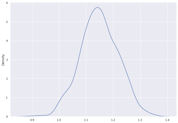
As we can see from plot, the distribution is somewhat Gaussian with \( \mu \approx 1.14 \). Most of the data points fall between 0.95 and 1.36, which gives a range of approximately \( \mu \pm 0.2 \). Now that we understand the noise better, we can account for that in our algorithm for obstacle avoidance.
while True:
  idx = 0
  robot.set_vel(1,0)
  hist = 6.0
  while robot.get_laser_data() > 0.3:
    time.sleep(0.02)
    if idx == 0:
      hist = robot.get_laser_data()
      idx = idx + 1
    if idx == 50:
      if abs(robot.get_laser_data()-hist) < 0.5 and hist != 6.0:
        break
      else:
        idx = 0
  dur = random.uniform(1,3)
  dire = random.random()
  if (dire < 0.45):
      robot.set_vel(-0.05, 2)
  elif (dire < 0.9):
      robot.set_vel(-0.05, -2)
  elif (dire < 0.95):
      robot.set_vel(-1, 0.5)
  else:
      robot.set_vel(-1, -0.5)
  time.sleep(dur)
First, the robot travels straight. Whenever the laser data drops below 0.3, which we know can be anything from 0.1 to 0.5 in the simulator, we have to change the course of our robot. Usually, that can be fixed by spinning in place. Therefore, we can randomly choose a direction and spin from 90 degrees to 270 degrees, which may or may not get us away from that obstacle. If not, we can always try again. We also assign a small negative linear velocity to slightly help the robot move away from the obstacle.
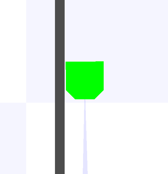
In rare circumstances, turning in place cannot fix the problem. For example, in the image below, there is no place for the robot to spin clockwise or counterclockwise. Therefore, two more actions are introduced. With a 10% chance, the robot might back up with a random direction. Since we check the robot every second, the robot can get out of this situation in a few seconds.
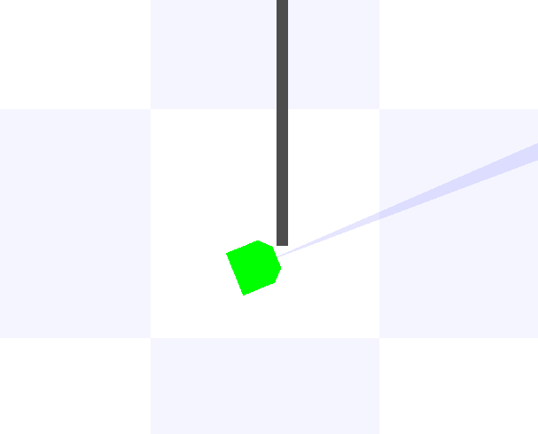
Getting stuck at corners is also something quite rare. As we can see from the picture below, the robot is stuck but the range finder provides no useful information due to its small detection angle. Therefore, our program also checks whether the range finder data has changed in the past second. Again, from the distributino plot above, we know that the maximum difference between two signals when the robot is stuck should be about 0.4, which is why the threshold is set to 0.5, just in case.
With these different scenarios in mind, the robot wanders on the map endlessly, or at least for half an hour or so before I shut it off, without getting stuck. Below is a short segment from the run.
We can actually see that the robot got stuck at the corner at about 0:18, and that the robot is able to free itself and return to normal. However, that is still considered a collision. In order to avoid collision completely, the robot cannot travel in a straight line as the limited detection angle will not be able to see corners or walls in parallel. To fix it, we either need to add more sensors, or spin a little so we can cover a larger angle.