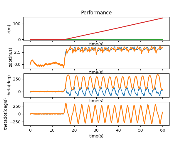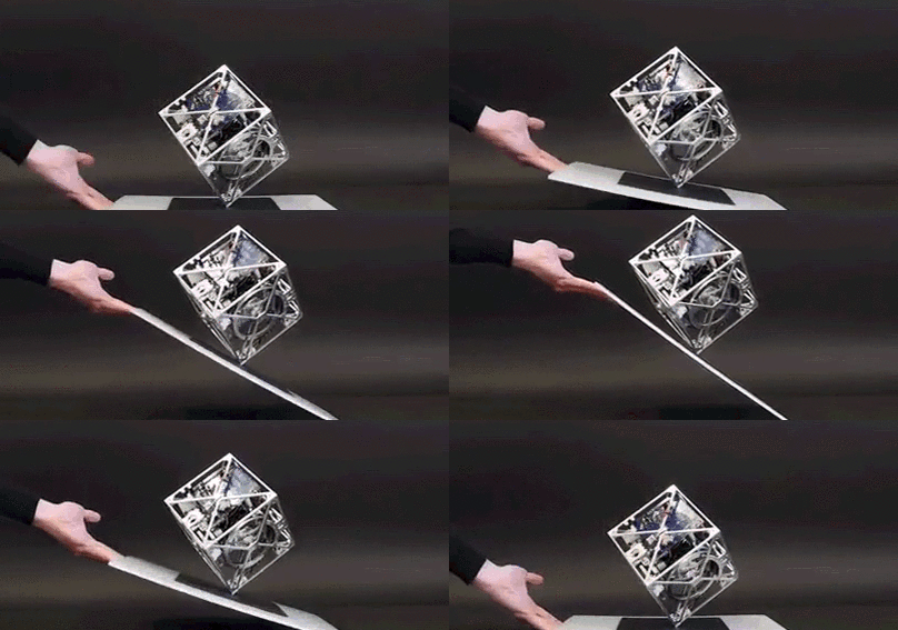
The objective of this lab is to experiment with the Kalman filter and see what effects different modifications on the model (noise, initial state, etc.) has on the inverted pendulum on a cart.
I downloaded the code and compared it with the one from lab 11. New A and B matrices in the Kalman filter version are discretized, and we are not measuring all state variables as the C matrix only has a one on the last column.
I ran the simulation, practically unchanged, with different reference waves.
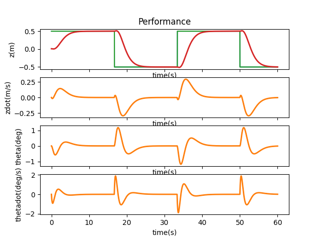
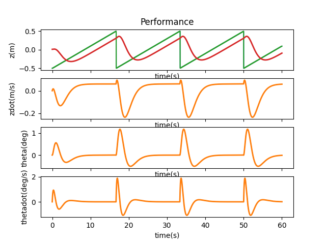
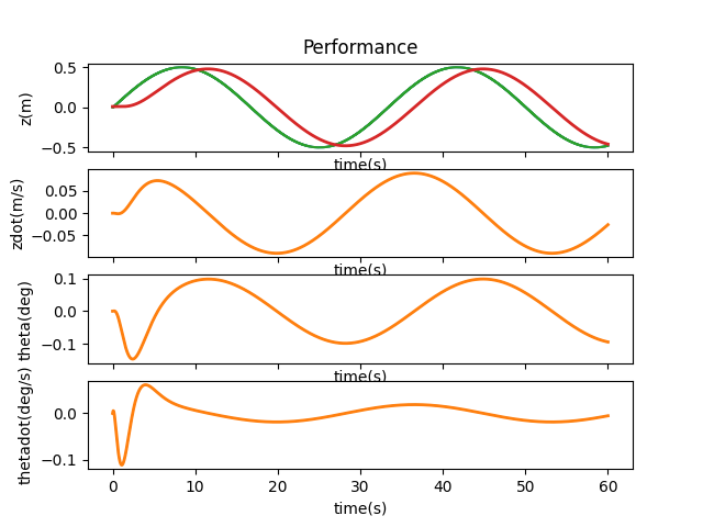
When I run control.obsv(P.A,P.C) and calculate the rank using np.linalg.matrix_rank, I get a result of 3, which is smaller than 4, the size of our state space, indicating that the system is not observable. Lookaing at matrices A and C as well as the observability matrix, it would seem like \( x \), or \( z \), would be the state that is not observable. By changing one initial state at a time, we can verify if the system is able to correct itself and therefore deduce which state is not observable.
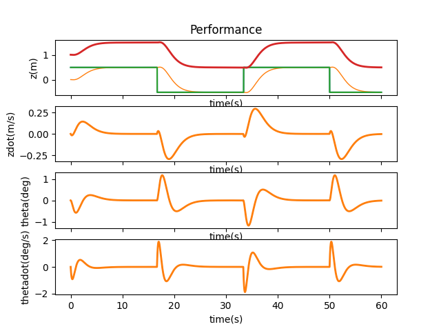
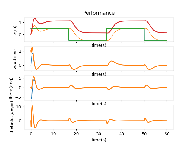
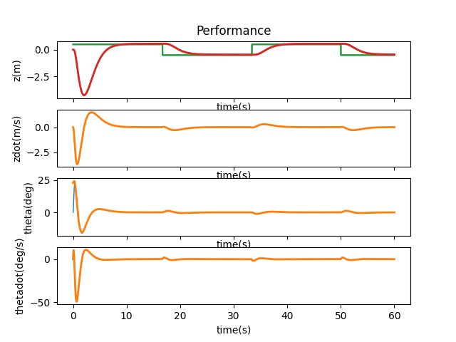
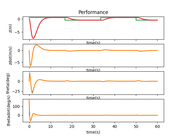
As we can see from the above plots, if $z$ is off, there is no way to correct it given our current system and the offset persists. Therefore, it is the state that is not observable. When the other states have an offset, they can either be directly or indirectly adjusted. For example, when $\theta$ has a different initial value, the cart is able to lift the pendulum back to upright position.
Next, to have a more realistic estimate of how well Kalman filter works, I added imperfections step by step.
First, some random noise are added to all four initial states as discrepencies. The Kalman filter seems to be able to adjust very quickly, even though it can’t get rid of the offset in $z$. The variance I chose for $z$ and $\dot{z}$ are $0.5$. For $\theta$, $20^\circ$ and for $\dot{\theta}$, $\frac{\pi}{2}rad/s$. These are all relatively high errors and the real offsets are unlikely to exceed the range.
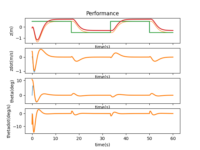
For the deadband and saturation, we know from lab 6 that the cart has a maximum acceleration of about $3m/s^2$. For the minimum acceleration, I decided on $0.2m/s^2$ because it seems resonable. This is honestly not great because drag is ignored.
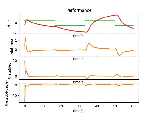
The overall balancing of the pendulum seems to be working fine, but the $z$ position unfortunately fails to be updated correctly. This is probably due to the deadband region. The cart tries to do tiny changes to adjust the position but the deadband region does not allow it to happen. Movements are therefore more jerky.
To add process noise, only a single line in the dynamic model has to be uncommented.
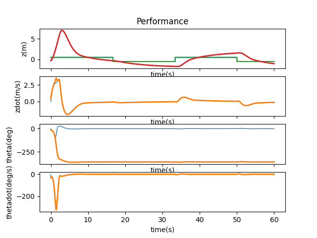
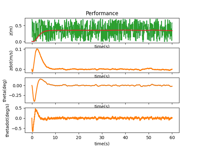
The process noise does not seem to make a lot of difference. Measurement noise is then accomplished by adding random values to the state values, or old_state, that are multiplied by matrix C at every iteration. As expected, the measurement noise has a huge impact on the Kalman filter result and I had to lower my original variance by a lot. I also found out that my initial state discrepency might have too big of an impact as all the modifications after it has a significant chance of breaking the system especially with the measurement noise added so I lowered the variance by 75%. Shown below is the result of a broken controller.

The cart just goes further and further to the right and never comes back. After adjusting, however, the system is a lot more stable. Still, the measurement noise cannot be too large. The final values I settled on was 0.1, which is about $6^\circ/s$.
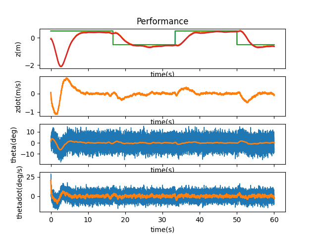
The system is still pretty stable even though the estimates are quite noisy.
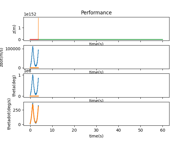
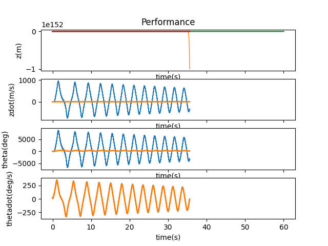
To modify matrices A and B, I decided to simply scale the matrices upwards until the systems starts breaking again. First, I only scaled A by 30%. The system went absolutely nuts. The cart literally flew out of the universe, and then some.
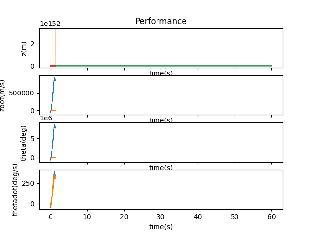
10% was no better.
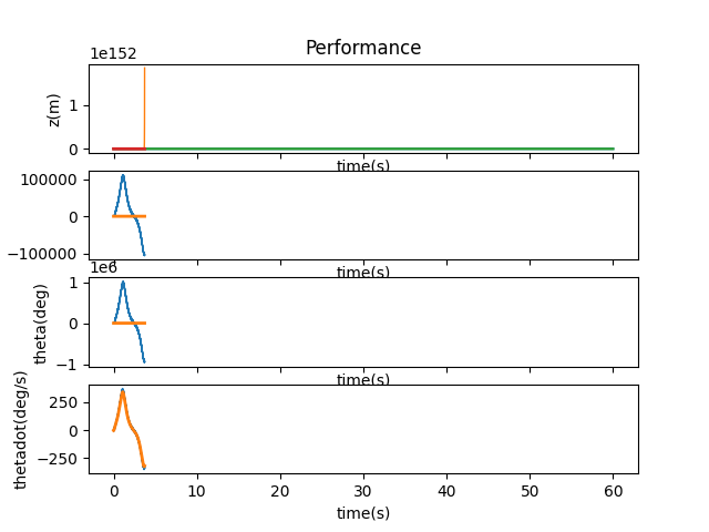
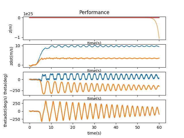
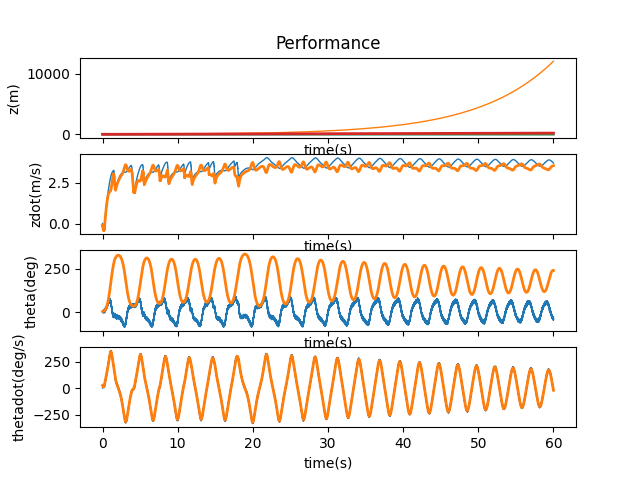
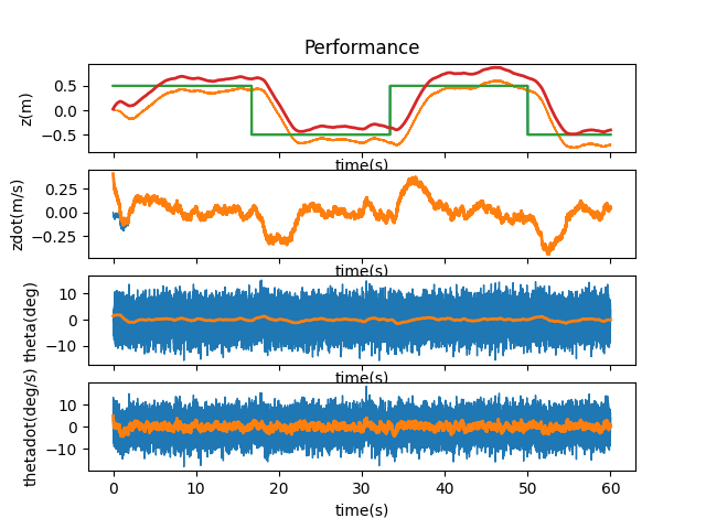
Finally, something that doesn’t break physics. I then tried to scale B in the same way. I learned my lesson and started trying at 0.1%.
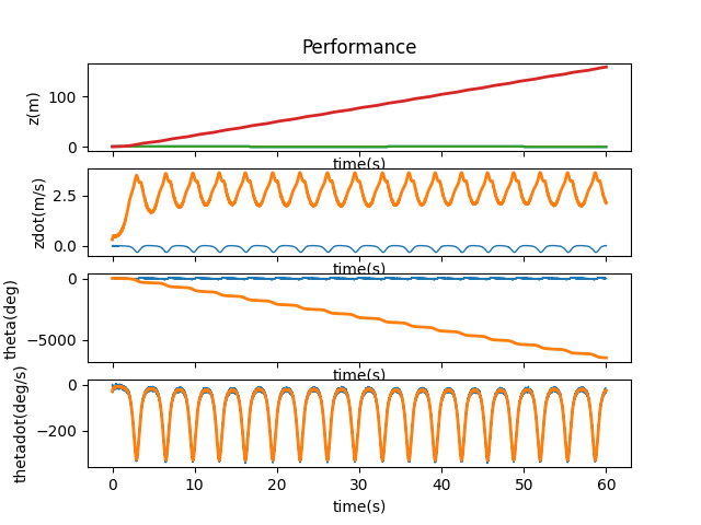
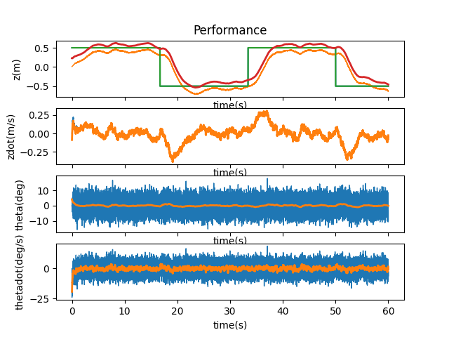
B seems to be a lot more forgiving. What if A and B are both changed by the values that work from above?
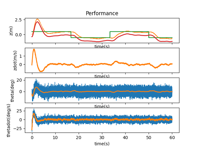
Lastly, let’s try changing the update time. First, from 1ms to 10ms.
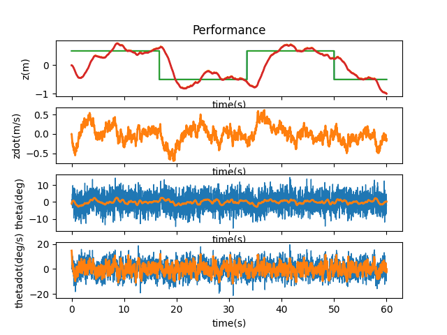
Honestly, I am surprised but glad that it worked. It is more jittery but if the actual robot performs like this I’ll be waking up from my sleep smiling. I then tried to find the maximum possible time.
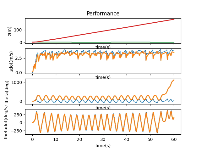
100ms unfortunately doesn’t work.
20ms, however, produces different results with different initial conditions.
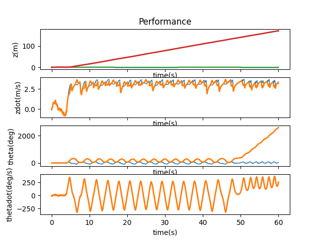
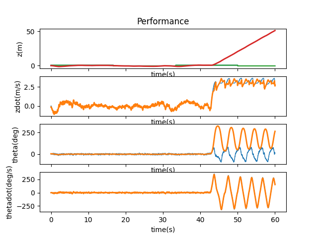
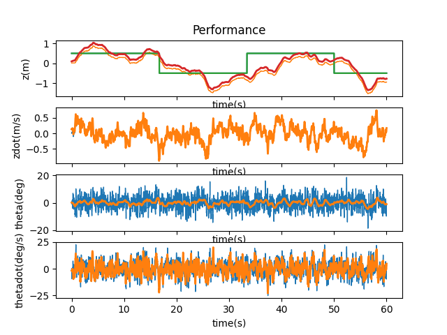
It seems that 10ms is about the limit.
With all the imperfections implemented, I think the robot MIGHT be able to do it. The biggest concern I have is the motors and I don’t believe that is remotely close to perfectly modeled through our simulation.
To incorporate the TOF sensor, I changed the C matrix and update y_kf at 100HZ. However, for 9 cycles out of 10, the $z$ measurement is replaced by a history value that is updated every 10 cycles. This would effectively mean we are measuring both $\dot{\theta}$ (at appr. 100Hz) and $z$ (at appr. 10Hz). After a few trials, however, it seems that incorporating the TOF sensor is counterproductive for some reason. It is possible that this happens because no measurements are better than laggy measurements, as the Kalman filter actually gets the outdated measurements for $z$ most of the time.
