Objective
The objective of this lab is to perform navigation from a random start point to a random end point by combining algorithms for path planning and and Bayes/odomtery for localization. As described in my lab 9 report, the restrictions in my apartment hinders the accuracy of my localization, therefore I decided to do this lab completely in the virtual simulator and create a much more interesting geometry that hopefully increases the accuracy of my Bayes filter.
Simulation
Since I am using the simulator only, I created a much more insteresting map loosely based on my apartment.
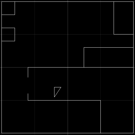
With two new trajectories, I tested out how good Bayes localization is.
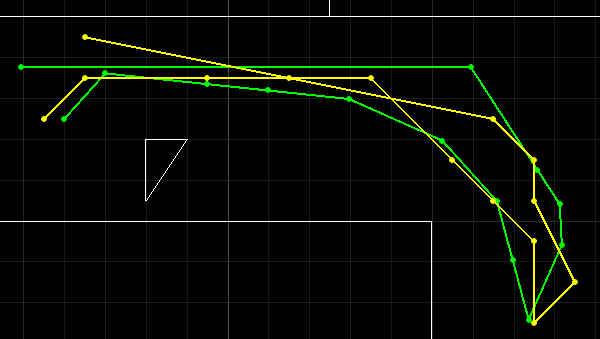
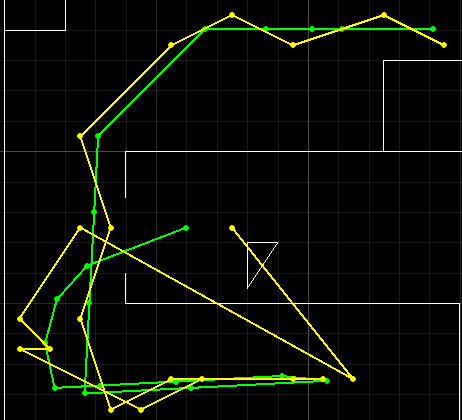
As we can see, the localization works relatively well, but there are still some outliers.
Occupancy Matrix
A way to represent my map is to convert it to an occupancy matrix with 1 representing the obstacles. To represent the robot as a point, proper clearance from the obstacles is also required. Therefore, I created an occupancy matrix with each grid representing a 0.1mx0.1m square with padding/clerance set to 0.3m. When converting line segments into occupany matrices, I simply find the distances between the line segment and the blocks nearby and set the ones below the threshold to 1. Below is the occupancy matrix generated with two random start points and two random goals. We will focus on these two because they present some interesting challenges.
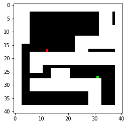
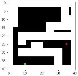
I explored two different algorithms in terms of time complexity and space complexity.
BFS
BFS assumes that all costs are equal. Therefore, the only logical moves are moving to the blocks directly adjacent to the current block.
def bfs(grid, start_cell, end_cell):
    frontier = [start_cell]
    parents = {}
    max_size = 0
    it1 = 0
    it2 = 0
    while(frontier):
        it1 = it1 + 1
        max_size = max(len(frontier),max_size)
        curr_node = frontier[0]
        frontier = frontier[1:]
        if (curr_node[0] == end_cell[0] and curr_node[1] == end_cell[1]):
            break
        for i in [(-1,0),(1,0),(0,-1),(0,1)]:
            new_node = curr_node + i
            if (new_node[0],new_node[1]) in parents or grid[new_node[0],new_node[1]] == 1:
                continue
            it2 = it2 + 1
            frontier.append(new_node)
            parents[(new_node[0],new_node[1])] = curr_node
    curr_node = end_cell
    backtrace = []
    while(curr_node[0] != start_cell[0] or curr_node[1] != start_cell[1]):
        backtrace.append(curr_node)
        curr_node = parents[(curr_node[0],curr_node[1])]
    print("max length of frontier is {}".format(max_size))
    print("it1 is {}".format(it1))
    print("it2 is {}".format(it2))
    return backtrace[::-1]
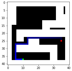
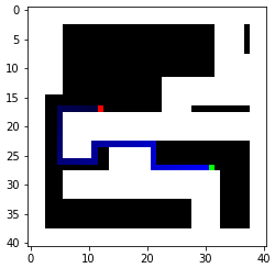
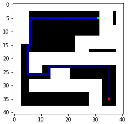
As we can see, BFS indeed finds the optimal Manhattan distance path. I also printed out some key stats, including the maximum frontier size, the amount of iterations, and the execution time averaged over five searches. The execution time is surprisingly good, likely because the frontier hits the obstacles and limits its size. Therefore, the algorithm does not have to search through a lot of nodes. The algorithm also does not have to do redundant work because a history of visited nodes is kept. This also reduces the memory required as the maximum length of all these different frontiers is only 24 (with the increased resolution).
| Index | 1 | 2 | 3 |
|---|---|---|---|
| Max Frontier | 13 | 24 | 20 |
| Iterations Big Loop | 289 | 609 | 680 |
| Iterations Small Loop | 299 | 612 | 681 |
| Avg. Exec Time (s) | 0.012 | 0.024 | 0.035 |
| Path Length (m) | 5.1 | 4.9 | 9.2 |
Dijkstra’s Algorithm
The most important distinction between BFS and Dijkstra’s algorithm is the addition of cost. We no longer have to assume equal cost, which means the robot can move diagonally or at any arbitrary angle. One advantage that Dijkstra’s algorithm has over A* is that it finds the optimal path with minimal cost. Even though it takes a little longer, it would be worth it as the time it takes for the robot to execute the path would be greater than the time it takes for extra computation. For simplicity, my implementation only explores the eight blocks directly connected to the current block.
def dijkstra(grid, start_cell, end_cell):
    frontier = [start_cell]
    parents = {}
    cost = {(start_cell[0],start_cell[1]): 0}
    max_size = 0
    it1 = 0
    it2 = 0
    while(frontier):
        it1 = it1 + 1
        max_size = max(len(frontier),max_size)
        min_i = 0
        min_d = cost[(frontier[0][0],frontier[0][1])]

        # If I keep the nodes sorted, I could get O(logn) insert and O(1) access
        # instead of O(n) access and O(1) insert but this is merely a proof of concept
        for i in range(len(frontier)):
            node = frontier[i]
            if cost[node[0],node[1]] < min_d:
                min_d = cost[node[0],node[1]]
                min_i = i
        curr_node = frontier.pop(min_i)
        if (curr_node[0] == end_cell[0] and curr_node[1] == end_cell[1]):
            break
        for i in [-1,0,1]:
            for j in [-1,0,1]:
                if (i == 0 and j == 0):
                    continue
                new_node = curr_node + (i,j)
                new_node = (new_node[0],new_node[1])
                new_c = cost[(curr_node[0],curr_node[1])]+(i**2+j**2)**0.5
                if new_node in cost:
                    if cost[new_node] <= new_c:
                        continue
                if grid[new_node] == 1:
                    continue
                if i != 0 and j != 0:
                    if grid[(new_node[0]-i,new_node[1])] == 1 or grid[(new_node[0],new_node[1]-j)] == 1:
                        continue
                it2 = it2 + 1
                frontier.append(np.array(new_node))
                parents[new_node] = curr_node
                cost[new_node] = new_c
    curr_node = end_cell
    backtrace = []
    while(curr_node[0] != start_cell[0] or curr_node[1] != start_cell[1]):
        backtrace.append(curr_node)
        curr_node = parents[(curr_node[0],curr_node[1])]
    print("max length of frontier is {}".format(max_size))
    print("it1 is {}".format(it1))
    print("it2 is {}".format(it2))
    return backtrace[::-1]
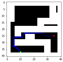
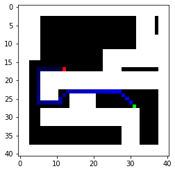
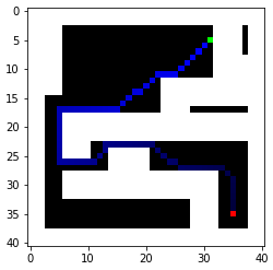
As we can see, Dijkstra’s algorithm does find the most optimal path with the given 8 options. To minimize execution time, my cost function could use a little improvement as right now it only accounts for the distance between two blocks but doesn’t account for the turning time. Regardless, the paths found by Dijkstra’s algorithm should be faster than the one found by BFS because of the diagonal route. Key stats are also found below compared to the BFS.
| Index | 1 | 2 | 3 |
|---|---|---|---|
| Max Frontier BFS | 13 | 24 | 20 |
| Max Frontier DIJ | 20 | 47 | 48 |
| Extra Space | 53.8% | 95.8% | 140% |
| Avg. Exec Time BFS | 0.012 | 0.024 | 0.035 |
| Avg. Exec Time DIJ | 0.029 | 0.054 | 0.063 |
| Extra Time | 142% | 125% | 80% |
| Path Length BFS | 5 | 4.8 | 9.1 |
| Path Length DIJ | 4.572 | 4.549 | 8.029 |
| Improvement | 8.56% | 5.23% | 11.8% |
It is worth noting that additional memory is required for both methods to keep track of other important data, such as parents (both) and cost (Dijkstra). Both only require a small amount of memory, fortunately.
Overall, I would say that Dijkstra’s algorithm is worth it because the computation time compared to the execution time is insignificant.
Open-loop Control
Since setting velocities on the simulator is precise, the easiest way to navigate would be open-loop control with a known start position. Indeed, the algorithms already provide detailed steps to be followed and all the robot has to do is to travel at a certain angle for a certain amount of time. For example, it could execute the third path created by both Dijkstra’s algorithm and BFS.
It seems like the BFS path actually takes a shorter amount of time. This is because the Dijkstra path spends too much time turning, and the virtual robot is better at travelling straight. The fix would be the solution I mentioned above, using travel time instead of distance as the cost so turning time would become part of the equation.